
Programming Exercise 7:
K-means Clustering and Principal Component Analysis
In this exercise, you will implement the K-means clustering algorithm and apply it to compress an image. In the second part, you will use principal component analysis to find a low-dimensional representation of face images. Before starting on the programming exercise, we strongly recommend watch- ing the video lectures and completing the review questions for the associated topics.
To get started with the exercise, you will need to download the starter code and unzip its contents to the directory where you wish to complete the exercise. If needed, use the cd command in Octave to change to this directory before starting this exercise.
Files included in this exercise
Throughout the first part of the exercise, you will be using the script ex7.m, for the second part you will use ex7 pca.m. These scripts set up the dataset for the problems and make calls to functions that you will write. You are only required to modify functions in other files, by following the instructions in this assignment.
K-means Clustering
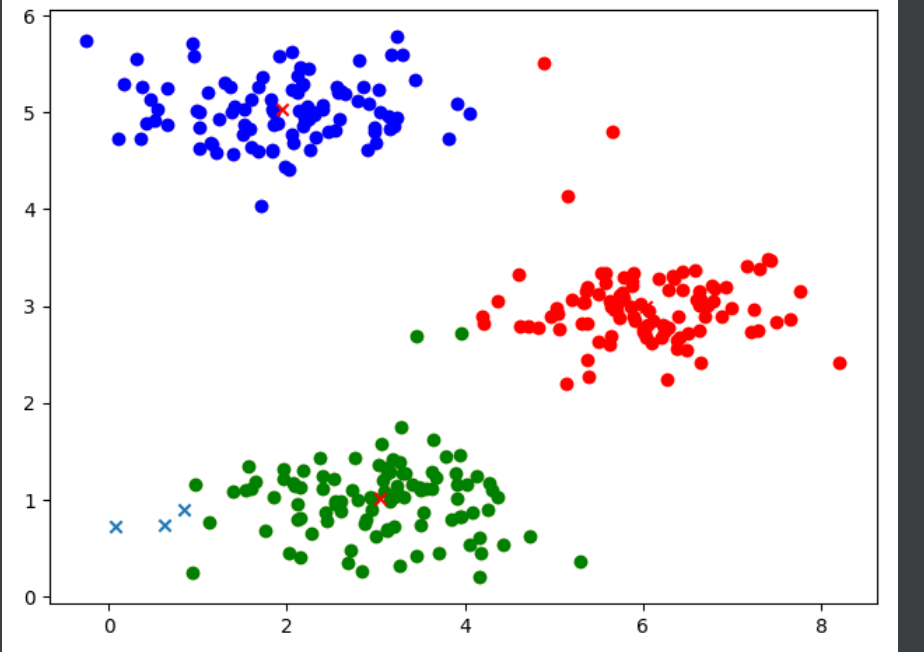
In this this exercise, you will implement the K-means algorithm and use it for image compression. You will first start on an example 2D dataset that will help you gain an intuition of how the K-means algorithm works. After that, you wil use the K-means algorithm for image compression by reducing the number of colors that occur in an image to only those that are most common in that image. You will be using ex7.m for this part of the exercise.
代码如下:
from scipy.io import loadmat
import numpy as np
from matplotlib import pyplot as plt
data = loadmat("ex7data2.mat")['X']
x = data.T[0]
y = data.T[1]
inix = np.random.rand(1,3)
iniy = np.random.rand(1,3)
mark=[]
plt.scatter(inix,iniy,marker='x')
def find_near():
l=[]
for i in range(x.size):
xp = x[i]
yp = y[i]
r=(((inix-xp)**2)+((iniy-yp)**2))[0]
l.append(np.where(r==np.min(r))[0][0])
return np.asarray(l)
def adjust_point(mark):
for i in range(iniy.size):
nx = np.mean(x[np.where(mark==i)])
ny = np.mean(y[np.where(mark==i)])
if np.isnan(nx):
continue
inix[0][i]=nx
iniy[0][i]=ny
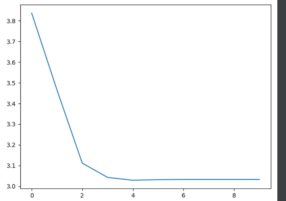
def cost(x,y,inix,iniy):
tlt=0
for i in range(len(inix[0])):
tlt=tlt+np.mean(np.sqrt((x-inix[0][i])**2+(y-iniy[0][i])**2))
return tlt/len(inix[0])
ct=[]
itcnt=10
for i in range(itcnt):
mark = find_near()
adjust_point(mark)
ct.append(cost(x,y,inix,iniy))
plt.scatter(x, y,alpha=0.5)
c = ['r','g','b']
for i in range(iniy.size):
nx = x[np.where(mark == i)]
ny = y[np.where(mark == i)]
plt.scatter(nx,ny,c=c[i])
plt.scatter(inix,iniy,marker='x',c='r')
plt.show()
cx=np.arange(0,itcnt)
plt.plot(cx,ct)
plt.show()效果如下:
代价函数如下:
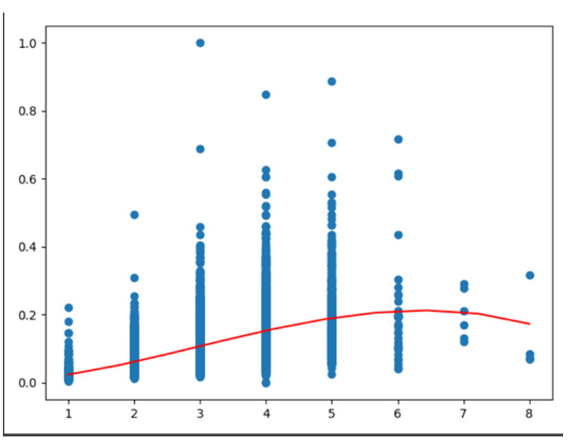
泰坦尼克号生存预测
主要问题:什么样的人在泰坦尼克号中更容易存活?
单单ROOM的因素
import numpy as np
from matplotlib import pyplot as plt
import pandas as pd
import scipy.optimize as opt
from sklearn.preprocessing import MinMaxScaler
#载入文件
from sklearn.preprocessing import PolynomialFeatures
data=pd.read_csv("python_dataset.csv")
#构建numpy矩阵
X = np.asarray(data.iloc[0:,0:1])
Y = np.asarray(data['Price'])
Y=(Y-Y.min())/(Y.max()-Y.min())
plt.scatter(X,Y)
poly_reg = PolynomialFeatures(degree=3)
X = poly_reg.fit_transform(X).T
def gradient(theta, X, y,lamda=1):
theta_n = theta[1:]
reg_theta = (lamda/len(X))*theta_n
reg_theta = np.concatenate((np.asarray([0]),reg_theta))
return (1 / len(X)) * np.dot(X,((h(X,theta)) - y).T) + reg_theta
#定义假设函数
def h(X,theta):
return np.sin(np.matmul(theta,X))/2
#定义代价函数
def costFunction(theta,X,Y):
inner = np.power(h(X,theta)-Y,2)
return np.sum(inner)/(2 * len(X[0]))
#初始化theta矩阵
theta = np.zeros([1,X.shape[0]])
#输出theta初始值的矩阵
print("Theta 为0的时候代价函数的值:",end='')
print(costFunction(theta,X,Y))
#cost数列用来存储每次训练的代价
cost=[]
#运用梯度下降来对函数拟合
def gradientDescent(X, y, theta, alpha, iters):
#开始迭代iters次
for i in range(iters):
#构建 h_theta(x^(i))-y 的值
error = (h(X,theta)-y)
#theta_tempy用来存储下一次的theta列表来实现同时更新
theta_temp=[[]]
#分别计算每一个theta的值
for j in range(len(theta[0])):
#计算 ( h_theta(x^(i))-y )· x_j 项
term = np.multiply(error,X[j])
#求出theta,sum即公式中的求和符号
n = theta[0][j]-(( alpha / len(X[0]))*np.sum(term))
#加入零临时序列中
theta_temp[0].append(n)
#将数列转化为numpy并更新到theta
theta_temp = np.asarray(theta_temp)
theta=theta_temp
#加入代价序列
cost.append(costFunction(theta,X,Y))
return theta
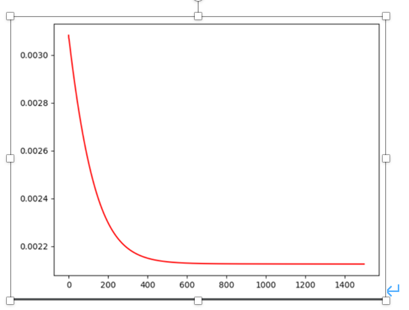
#alpha是学习率,iters是迭代次数
alpha=0.001
iters=1500
#开始梯度下降拟合函数
g = gradientDescent(X, Y, theta, alpha, iters)
print("Theta 拟合后时候代价函数的值:",end='')
print(costFunction(g,X,Y))
# res = opt.minimize(fun=costFunction, x0=theta, args=(X, Y), jac=gradient,method='TNC',)
# print(res)
# g=np.asarray([res.x])
#画出图像
#打印出散点图和拟合后的直线
x=np.linspace(X[1].min(),X[1].max(),10).reshape((10,1))
x=poly_reg.fit_transform(x).T
y = np.sin(g @ x)/2
x=np.linspace(X[1].min(),X[1].max(),10).reshape((10,1))
plt.plot(x.T[0],y[0],'r')
plt.show()
#打印出代价函数的变化曲线
t = np.arange(iters)
plt.plot(t,cost,'r')
plt.show()结果如下:
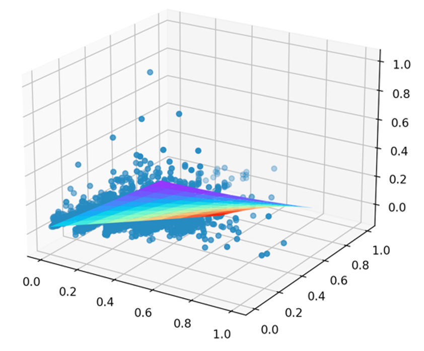
ROOM with Distance的因素
import numpy as np
import pandas as pd
from matplotlib import pyplot as plt
from mpl_toolkits.mplot3d import Axes3D
#import scipy.optimize as opt
#载入文件
data=pd.read_csv("python_dataset.csv")
#构建numpy矩阵
data.insert(0,'one',1)
X = np.asarray(data.iloc[0:,0:3]).T
for i in range(1,len(X)):
X[i]=(X[i]-X[i].min())/(X[i].max()-X[i].min())
X = np.concatenate((X,[X[1]*X[2]],[(X[1]**2)*X[2]],[(X[2]**2)*X[1]]))
Y = np.asarray(data['Price'])
Y=(Y-Y.min())/(Y.max()-Y.min())
fig = plt.figure()
ax = Axes3D(fig)
ax.scatter(X[1],X[2],Y,zdir='z')
def gradient(theta, X, y,lamda=1):
theta_n = theta[1:]
reg_theta = (lamda/len(X))*theta_n
reg_theta = np.concatenate((np.asarray([0]),reg_theta))
return (1 / len(X)) * np.dot(X,((h(theta,X)) - y).T) + reg_theta
#定义假设函数
def h(theta,X):
return np.matmul(theta,X)
# #定义代价函数
def costFunction(theta,X,Y):
inner = np.power(h(theta,X)-Y,2)
return np.sum(inner)/(2 * len(X[0]))
# #初始化theta矩阵
theta = np.zeros([1,X.shape[0]])
# #输出theta初始值的矩阵
print("Theta 为0的时候代价函数的值:",end='')
print(costFunction(theta,X,Y))
#
#
# #cost数列用来存储每次训练的代价
cost=[]
# #运用梯度下降来对函数拟合
def gradientDescent(X, y, theta, alpha, iters):
#开始迭代iters次
for i in range(iters):
#构建 h_theta(x^(i))-y 的值
error = (h(theta,X)-y)
#theta_tempy用来存储下一次的theta列表来实现同时更新
theta_temp=[[]]
#分别计算每一个theta的值
for j in range(len(theta[0])):
#计算 ( h_theta(x^(i))-y )· x_j 项
term = np.multiply(error,X[j])
#求出theta,sum即公式中的求和符号
n = theta[0][j]-(( alpha / len(X[0]))*np.sum(term))
#加入零临时序列中
theta_temp[0].append(n)
#将数列转化为numpy并更新到theta
theta_temp = np.asarray(theta_temp)
theta=theta_temp
#加入代价序列
cost.append(costFunction(theta,X,Y))
return theta
#alpha是学习率,iters是迭代次数
alpha=0.1
iters=30000
#
# #开始梯度下降拟合函数
g = gradientDescent(X, Y, theta, alpha, iters)
print("Theta 拟合后时候代价函数的值:",end='')
print(costFunction(g,X,Y))
# res = opt.minimize(fun=costFunction, x0=theta, args=(X, Y), jac=gradient,method='TNC')
# g=res.x
# print(res)
#x: array([ 0.0341108 , 0.48157589, -0.17348541, -0.27254023, -0.71858818,
# 0.47850217])
# g=np.asarray([res.x])
# #画出图像
theta = np.asarray([g])
theta0 = np.arange(0, 1, 0.1)
theta1 = np.arange(0, 1, 0.1)
theta0,theta1 = np.meshgrid(theta0, theta1)
theta0 = np.ravel(theta0)
theta1 = np.ravel(theta1)
xt = np.asarray([[1]*len(theta0),theta0,theta1,theta1*theta0,(theta1**2)*theta0,(theta0**2)*theta1])
z = h(theta,xt).reshape(10,10)
theta0 = np.arange(0, 1, 0.1)
theta1 = np.arange(0, 1, 0.1)
theta0,theta1 = np.meshgrid(theta0, theta1)
ax.plot_surface(theta0,theta1,z,cmap='rainbow')
plt.show()
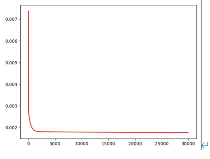
#打印出代价函数的变化曲线
t = np.arange(iters)
plt.plot(t,cost,'r')
plt.show()效果如下:
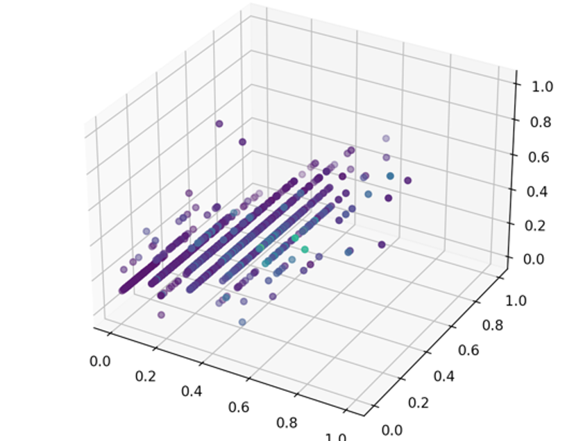
Room and Distence and bedroom
代码如下:
import numpy as np
import pandas as pd
from matplotlib import pyplot as plt
from mpl_toolkits.mplot3d import Axes3D
import scipy.optimize as opt
#载入文件
from sklearn.preprocessing import PolynomialFeatures
data=pd.read_csv("python_dataset.csv")
#构建numpy矩阵
X = np.asarray(data.iloc[0:,0:2]).T
for i in range(0,len(X)):
X[i]=(X[i]-X[i].min())/(X[i].max()-X[i].min())
n = np.asarray(data['Bedroom2'])
n=(n-n.min())/(n.max()-n.min())
X = np.concatenate((X,[n]))
poly_reg = PolynomialFeatures(degree=3)
P = poly_reg.fit_transform(X.T).T
Y = np.asarray(data['Price'])
Y=(Y-Y.min())/(Y.max()-Y.min())
fig = plt.figure()
ax = Axes3D(fig)
ax.scatter(X[0],X[1],X[2],c=Y,cmap="viridis",zdir='z')
plt.show()
def gradient(theta, X, y,lamda=1):
theta_n = theta[1:]
reg_theta = (lamda/len(X))*theta_n
reg_theta = np.concatenate((np.asarray([0]),reg_theta))
return (1 / len(X)) * np.dot(X,((h(theta,X)) - y).T) + reg_theta
#定义假设函数
def h(theta,X):
return np.matmul(theta,X)
# #定义代价函数
def costFunction(theta,X,Y):
inner = np.power(h(theta,X)-Y,2)
return np.sum(inner)/(2 * len(X[0]))
# #初始化theta矩阵
theta = np.zeros([1,P.shape[0]])
#
#输出theta初始值的矩阵
print("Theta 为0的时候代价函数的值:",end='')
print(costFunction(theta,P,Y))
# #
# #
# # #cost数列用来存储每次训练的代价
cost=[]
# # #运用梯度下降来对函数拟合
def gradientDescent(X, y, theta, alpha, iters):
#开始迭代iters次
for i in range(iters):
#构建 h_theta(x^(i))-y 的值
error = (h(theta,X)-y)
#theta_tempy用来存储下一次的theta列表来实现同时更新
theta_temp=[[]]
#分别计算每一个theta的值
for j in range(len(theta[0])):
#计算 ( h_theta(x^(i))-y )· x_j 项
term = np.multiply(error,X[j])
#求出theta,sum即公式中的求和符号
n = theta[0][j]-(( alpha / len(X[0]))*np.sum(term))
#加入零临时序列中
theta_temp[0].append(n)
#将数列转化为numpy并更新到theta
theta_temp = np.asarray(theta_temp)
theta=theta_temp
#加入代价序列
cost.append(costFunction(theta,X,Y))
return theta
# #alpha是学习率,iters是迭代次数
alpha=0.1
iters=3000
# #
# #开始梯度下降拟合函数
g = gradientDescent(P, Y, theta, alpha, iters)
print("Theta 拟合后时候代价函数的值:",end='')
print(costFunction(g,P,Y))
#
# res = opt.minimize(fun=costFunction, x0=theta, args=(P, Y), jac=gradient,method='TNC')
# g=res.x
# print(res)
x1 = np.linspace(0,1,10)
x2 = np.linspace(0,1,10)
x3 = np.linspace(0,1,10)
x1,x2,x3=np.meshgrid(x1,x2,x3)
y=[]
i=np.ravel(x1)
j=np.ravel(x2)
k=np.ravel(x3)
for m in range(len(i)):
l=np.asarray([[i[m],j[m],k[m]]])
P = poly_reg.fit_transform(l).T
y.append(h(g,P))
ax.scatter(x1,x2,x3,c=y,cmap="viridis",zdir='z')
plt.show()
# # g=np.asarray([res.x])
# # #画出图像
# theta = np.asarray([g])
# theta0 = np.arange(0, 1, 0.1)
# theta1 = np.arange(0, 1, 0.1)
# theta0,theta1 = np.meshgrid(theta0, theta1)
# theta0 = np.ravel(theta0)
# theta1 = np.ravel(theta1)
# xt = np.asarray([[1]*len(theta0),theta0,theta1,theta1*theta0,(theta1**2)*theta0,(theta0**2)*theta1])
# z = h(theta,xt).reshape(10,10)
# theta0 = np.arange(0, 1, 0.1)
# theta1 = np.arange(0, 1, 0.1)
# theta0,theta1 = np.meshgrid(theta0, theta1)
#
# ax.plot_surface(theta0,theta1,z,cmap='rainbow')
# plt.show()
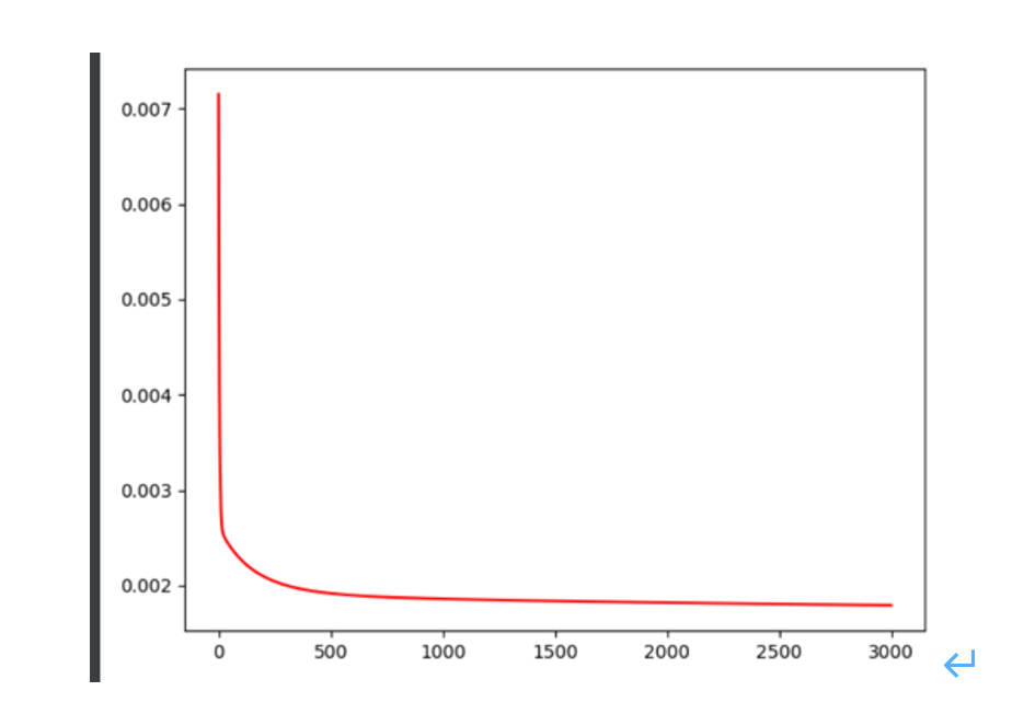
#打印出代价函数的变化曲线
t = np.arange(iters)
plt.plot(t,cost,'r')
plt.show()效果如下:
留言